Creating Multi-panel plots with hermpy

This example demonstrates how to construct multi-panel time series plots using hermpy.plotting.MultiPanel. We fetch one hour of MESSENGER MAG and FIPS data, parse them into their respective data structures, and progressively build up a combined plot.

import xarray as xr
from astropy.table import QTable
from sunpy.time import TimeRange

from hermpy.data import fips_energy_bin_edges, parse_messenger_fips, parse_messenger_mag
from hermpy.net import ClientMESSENGER
from hermpy.plotting import MultiPanel, SpectrogramPanel, TimeseriesPanel

First we must get some data. Here we fetch MESSENGER MAG and FIPS data for a particular time range.

We use hermpy.net.ClientMESSENGER to download MAG and FIPS data for a one-hour window. See here for more details.

c = ClientMESSENGER()
time_range = TimeRange("2011-09-26T12:00", "2011-09-26T13:20")

c.query(time_range, "MAG")
mag_file_paths = c.fetch()

c.query(time_range, "FIPS")
fips_file_paths = c.fetch()

We use Astropy’s Quantity Table (QTable) for time series data, and Xarray’s Dataset for 2D data. These custom parsers are included in hermpy.data, but may be replaced in later versions.

mag_data: QTable = parse_messenger_mag(mag_file_paths, time_range)
fips_data: xr.Dataset = parse_messenger_fips(fips_file_paths, time_range)

print(mag_data)

         UTC            X MSO     Y MSO     Z MSO      Bx      By      Bz
                          km        km        km       nT      nT      nT
--------------------- --------- --------- --------- ------- ------- --------
2011:269:12:00:00.020  -694.014   270.261  2615.208  231.18  -90.02 -393.552
2011:269:12:00:00.070  -694.192   270.249  2615.151 231.216  -90.01 -393.497
2011:269:12:00:00.120   -694.37   270.236  2615.094 231.344 -89.997 -393.423
2011:269:12:00:00.170  -694.548   270.224  2615.037 231.299 -89.997 -393.432
2011:269:12:00:00.220  -694.725   270.212   2614.98  231.38 -90.031 -393.358
2011:269:12:00:00.270  -694.903     270.2  2614.923 231.436 -90.084 -393.386
2011:269:12:00:00.320  -695.081   270.187  2614.865 231.435 -90.129 -393.378
2011:269:12:00:00.370  -695.259   270.175  2614.808 231.462 -90.063 -393.285
2011:269:12:00:00.420  -695.436   270.163  2614.751 231.507 -90.061 -393.276
                  ...       ...       ...       ...     ...     ...      ...
2011:269:13:19:59.520 -4028.764 -1001.012 -7865.931  17.683 -31.612    9.403
2011:269:13:19:59.570  -4028.74  -1001.02  -7866.01  18.151 -31.894    9.629
2011:269:13:19:59.620 -4028.717 -1001.028 -7866.089  18.667 -32.477    9.526
2011:269:13:19:59.670 -4028.693 -1001.036 -7866.168  19.133 -32.269    9.143
2011:269:13:19:59.720 -4028.669 -1001.044 -7866.247  18.947 -32.292    9.187
2011:269:13:19:59.770 -4028.646 -1001.052 -7866.326   18.48 -32.564    9.589
2011:269:13:19:59.820 -4028.622  -1001.06 -7866.405  17.875 -33.005    9.518
2011:269:13:19:59.870 -4028.599 -1001.068 -7866.484  17.596 -33.129    9.453
2011:269:13:19:59.920 -4028.575 -1001.076 -7866.563  17.919 -32.636   10.211
2011:269:13:19:59.970 -4028.551 -1001.084 -7866.642  17.822 -32.221   10.819
Length = 95995 rows

print(fips_data)

<xarray.Dataset> Size: 541kB
Dimensions:          (UTC: 505, Energy Channel: 63, Mode: 3407)
Coordinates:
  * UTC              (UTC) datetime64[us] 4kB 2011-09-26T12:00:02.262000 ... ...
  * Energy Channel   (Energy Channel) int64 504B 0 1 2 3 4 5 ... 58 59 60 61 62
  * Mode             (Mode) int64 27kB 2 2 2 2 2 2 2 2 2 2 ... 2 2 2 2 2 2 2 2 2
Data variables:
    Proton Flux      (UTC, Energy Channel) float64 255kB 0.0 0.0 0.0 ... 0.0 0.0
    Non-Proton Flux  (UTC, Energy Channel) float64 255kB 0.0 0.0 0.0 ... 0.0 0.0

As MESSENGER MAG data contains both ephemeris and magnetic field data, adding this data as it is to a Panel object will result in an error, as the columns (excluding the time column) have multiple units, and hence can’t be represented on the same axis.

We therefore need to shorten this table to just the columns we want in this Panel object.

mag_data.keep_columns(["UTC", "Bx", "By", "Bz"])

hermpy provides the Panel abstract base class, which is expanded upon in TimeseriesPanel and SpectrogramPanel.

We use a TimeseriesPanel as this matches the data type.

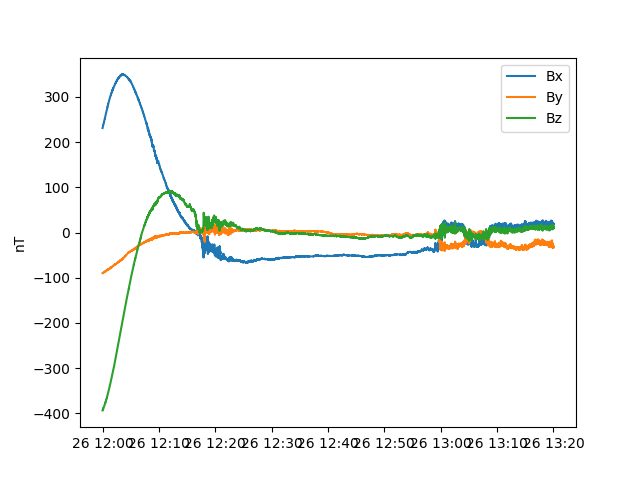
Each panel has a built-in plot function which returns a Figure and Axes for that panel in isolation. plt.show() is called within this function however uou can defer rendering until later by setting .plot(show=False), and then using plt.show() at a later point.

mag_panel = TimeseriesPanel(mag_data)
fig, ax = mag_panel.plot()

Plotting with more than one panel

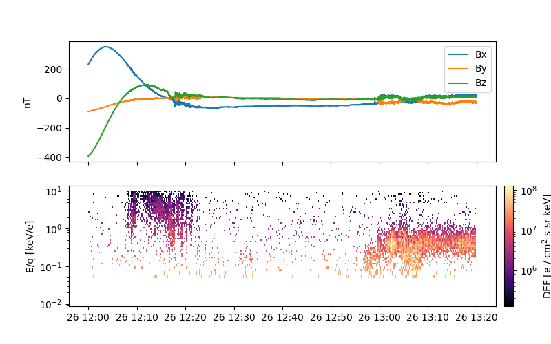
The power in Panel objects comes when we go to construct multipanel plots. We can combine Panel objects to construct a multi-panel plot by simply adding them.

Lets make a second panel where we plot the FIPS data. We can combine the two using the addition operator. SpectrogramPanel doesn’t know anything about our data, so we need to provide the time axis, y axis, and y bin edges.

proton_flux = fips_data["Proton Flux"]
fips_panel = SpectrogramPanel(
    proton_flux,
    time_dim="UTC",
    y_dim="Energy Channel",
    y_bin_edges=fips_energy_bin_edges(),
    cmap="magma",
    unit="DEF [e / cm$^2$ s sr keV]",
)

We can set anything about the plot with ax_set_params

fips_panel.ax_set_params = {"ylabel": "E/q [keV/e]"}

multipanel: MultiPanel = mag_panel + fips_panel
fig, axes = multipanel.plot()

You can also add multipanels to the same effect, and panels can also be added to multipanel objects.

multipanel += multipanel
multipanel.plot()

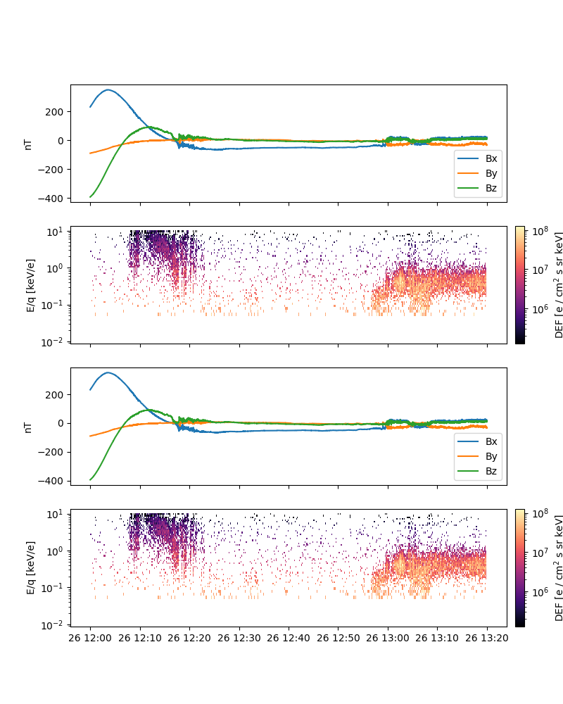
(<Figure size 800x1000 with 4 Axes>, array([<Axes: ylabel='nT'>, <Axes: ylabel='E/q [keV/e]'>,
       <Axes: ylabel='nT'>, <Axes: ylabel='E/q [keV/e]'>], dtype=object))

multipanel += mag_panel
multipanel.plot()

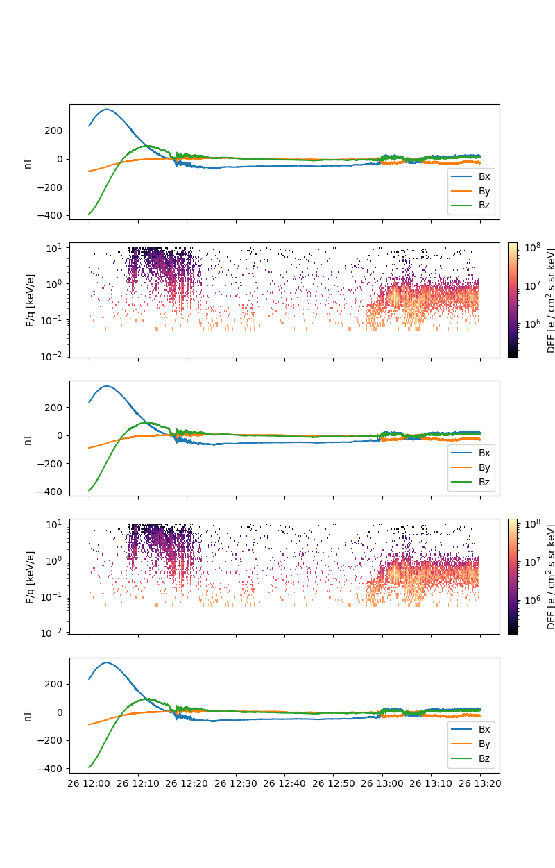
(<Figure size 800x1250 with 5 Axes>, array([<Axes: ylabel='nT'>, <Axes: ylabel='E/q [keV/e]'>,
       <Axes: ylabel='nT'>, <Axes: ylabel='E/q [keV/e]'>,
       <Axes: ylabel='nT'>], dtype=object))